
Every time you ask something of a chatbot, a semantic search engine or a shop’s recommender, there is no keyword matching going on underneath. Your sentence has been turned into a vector: a list of between 768 and 1536 decimal numbers — what the industry calls an embedding — that places its meaning in a space of more than a thousand dimensions. What gets searched are the stored vectors pointing in a similar direction. The interesting question is not that one, but another: how do you find them among a billion vectors without walking through them all?
Comparing against everything is not an option
The obvious method is called exact nearest neighbour search, and it means computing the distance between the query and every stored vector. With a million 1536-dimensional vectors that is 1.5 billion multiply-adds, which a modern CPU settles in a few tenths of a second. With a billion, the same computation runs into seconds and stops being viable for an interface that answers live.
The classic alternative was partitioning trees, such as the kd-tree: they split space into halves along whichever axis spreads the points most, discarding whole branches. In two or three dimensions they work beautifully. In 1536 they collapse: in such a space almost every point sits at almost the same distance from every other, and any boundary you draw cuts through most of the candidates. This is the well-known curse of dimensionality, and it explains why the industry accepted giving up exact answers.
A map with shortcuts
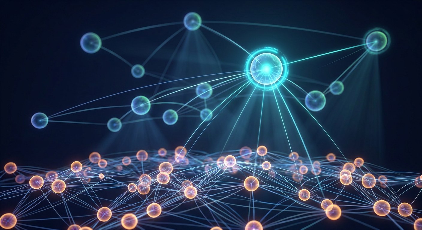
What is used today is approximate nearest neighbour search (ANN): you accept that one or two of every ten results will not be the optimal ones, in exchange for dropping from seconds to milliseconds. The trick is not to use lists but a graph. Each vector is a node, wired to its close neighbours. If only local connections existed, a query landing far away would have to hop node by node hundreds of times; so each node also keeps a few long-range links, chosen at random. That is a navigable small-world graph: you enter at any point and, at each step, jump to the neighbour closest to the query until no jump improves the distance. A handful of hops is enough to cross the entire space.
The hierarchy: motorways and streets
Today’s dominant algorithm, HNSW (Hierarchical Navigable Small World), adds a simple and highly effective idea: several stacked layers. The top layer holds a handful of widely separated vectors — the motorway network. Each layer below roughly doubles the number of nodes, and layer zero holds them all. When a vector is inserted it is given a random height with decreasing probability, so only a tiny fraction ever reaches the top.
Searching exploits that structure in two phases. First a greedy descent from the top layer: you move through those motorway nodes until you reach the right region of the space. Then, on layer zero, a beam search with a candidate list of size efSearch: instead of committing to a single route, several promising options are kept open, and the k nearest neighbours among all of them are returned. In real indexers, querying a one-million-vector index with a moderate setting costs under a millisecond and recovers more than 95% of the true neighbours for every ten results requested.
Four knobs
HNSW does not have many parameters, but each one settles a specific trade-off. M is how many links each node keeps, typically between 16 and 64; more links improve the quality of the map and make every hop and every byte of memory more expensive. efConstruction is the size of the candidate list during indexing, between 200 and 500: the larger it is, the better the graph turns out and the longer it takes to build. efSearch is chosen at query time and is the most convenient lever, because raising it improves accuracy without reindexing anything, at the sole cost of latency. And then the metric: cosine similarity, dot product or Euclidean distance give different results depending on how the embedding model was trained, and getting this one wrong ruins an otherwise perfect index.
The real bottleneck is memory
Storing a billion 1536-dimensional vectors in 32-bit floating point means more than six terabytes of data alone, plus the graph links: at M equal to 16 that is about 128 bytes per node, another 128 gigabytes. That is why compression is not decoration. Scalar quantization reduces each component to an 8-bit integer and cuts the footprint to a quarter with a small loss of precision. Product quantization is more aggressive: it splits the vector into subvectors — 96 blocks of 16 dimensions, say — and replaces each block with the identifier of the nearest centroid from a learned dictionary. Every vector drops from 6 kilobytes to about 96 bytes, 64 times less. Because the quantization code is approximate, the system retrieves a few hundred candidates using the compressed version and only re-ranks them with the full vectors, read back from disk.
That is where DiskANN comes from, the family of indexes that lives on SSD: it keeps approximate distances in memory and the graph on solid state, so each query triggers a few thousand random reads. It is the approach that makes searching billions of vectors profitable without a gigantic memory cluster.
Filtering without breaking the search
In production you are almost never searching the whole index: you search inside a subset (“only this customer’s documents”, “only this year’s articles”). Filtering before searching is exact but destroys performance, because the search can no longer hop across the graph. Filtering afterwards is fast but returns fewer results than requested, since the filter applies to just a few candidates. Today’s answer is to fold the condition into the traversal itself: every node is checked against the predicate first and the descent continues only among those that satisfy it, accepting that quality drops when the filter is very selective. Many systems also combine two retrievers — the vector one and a keyword index such as BM25 — and fuse both lists with a formula like Reciprocal Rank Fusion, which adds up reciprocals of the positions. That is hybrid search, and it usually beats either method on its own.
Seen this way, the feeling that a machine “understands” what you ask rests on something quite down to earth: four bytes per dimension, a graph with random shortcuts and a search that accepts being slightly wrong. The rest is scale.