
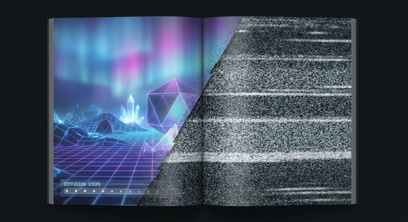
When an image model generates a portrait from the phrase “a lighthouse on a cliff in the fog”, it does not draw anything. There are no strokes, no brushes, no edges placed one after another. What it does is far stranger and far more elegant: it starts with an image of random noise, the same kind as the static on an old television set, and cleans it up over dozens of steps until a lighthouse emerges from the noise. The trick is that this cleanup is not a generic filter: it is the result of having learned to reverse a process that is genuinely easy to define mathematically.
Going forward is trivial: just add dirt
The core of these systems, called diffusion models, is a forward process that destroys an image over a series of steps. If x0 is the original image, step one adds a little Gaussian noise to produce x1, step two dirties x1 to produce x2, and so on up to xT, which is pure noise. Each step adds a small amount of noise controlled by a schedule of βt values that grow over time.
The beautiful part is that this process has a closed form. There is no need to simulate a thousand steps to know what the image looks like at step 400; it can be computed directly:
x_t = √(ᾱt) · x_0 + √(1 − ᾱt) · ε, with ε ~ N(0, I)
The factor ᾱt (cumulative alpha) is a running tally of how much of the original signal survives step t. At the start it is close to 1 and the image is still recognisable; at the end it is close to 0 and only noise remains. This formula is what makes everything else workable: it lets you pick any noise level at random and build the matching training example in a single operation.
Training means learning to guess the noise that was added
The network being trained, called εθ (usually a U-Net with skip connections or, since 2023, a Diffusion Transformer), receives three things: the noisy image xt, the step number t, and the conditioning (the text, a pose, a mask). Its task is a single one: to predict the exact noise that was added to reach that state.
Training is therefore almost offensively simple. Take an image from the dataset, draw a step t at random, generate the noise, and ask the model to guess it. The error is the mean squared distance between the real noise and the predicted one:
L = E[ || { & } ;epsilon; − εθ(x_t, t, c) ||{ & } ;sup2; ]
There is a theoretical result behind why this works: the function that best predicts the noise is proportional to the score (the gradient of the logarithm of the probability density) of the image distribution at each noise level. In other words, the model does not learn a recipe for drawing; it learns the direction in which the most probable image is pushing. Predicting noise, estimating the score and learning a vector field that pulls images back towards their natural distribution are three ways of saying the same thing.
Walking the path backwards, where it gets hard
Generating an image means reversing the process: start from pure noise and take steps backwards. Each step needs an estimate of the conditional distribution of the previous state. The original version (DDPM, 2020) used a stochastic rule that injected fresh randomness at every iteration, like someone retracing a staircase in small jumps. It needed between 500 and 1000 steps, which is why it was so expensive.
Modern variants reframe the walk as solving a differential equation (DDIM, the DPM-Solver, the Heun sampler). Turning it into a deterministic problem reaches the same quality in 20 or 50 steps instead of a thousand. A second-order DPM-Solver step does not cost much more than an Euler step, but it advances along a much straighter curve. And when generation has to happen in four steps or even one, distillation takes over: a small model is trained to imitate what the big master would do over several steps (consistency models, progressive distillation).
The shortcut that cut the cost: don’t diffuse over pixels
Adding noise and cleaning it directly on a 1024×1024 pixel image means the network handles millions of values in each of 50 steps, and spends most of its effort on details that are barely visible. The fix, introduced by Stable Diffusion in 2022, was to split the problem in two: a variational autoencoder (VAE) that compresses the image into a latent space of lower resolution (typically eight times smaller on each axis, with more channels), and the diffusion model itself, which works entirely inside that latent. A decoder then turns the result back into pixels.
The numbers explain the success: a 1024×1024×3 image holds about three million values; its latent holds around 200,000. Attention cost grows with the square of the number of elements, so reducing the internal resolution of the problem dramatically changes what fits on a graphics card. The trade-off is that the decoder sets a ceiling on sharpness, which is why final touch-ups often go through a separate stage or a super-resolution model.
How the text gets in: cross-attention and guidance without a classifier
The sentence you write is processed by a text encoder (CLIP, T5 or a large language model) and comes out as vectors. The diffusion network injects them into every block through cross-attention: the same mechanism that in a language model lets each token look at the others, except here the queries come from the elements of the latent image and the keys and values come from the text. That way, the region beginning to look like “water” can receive more influence from the word “water”.
With the trained model, generating an image conditioned on text alone gives rather soft results: the conditional prediction tends to be blurry. The standard fix is classifier-free guidance, a game of two predictions: one with the text and one without it (or with an empty prompt). The difference between them is amplified by a factor w:
ε = εno text + w · ( εwith text − εno text )
If w is 1, the result follows the prompt faithfully but looks flat; if w climbs to 12, the image becomes saturated, with burnt colours and strange anatomies, because the model is moving away from the natural variety of images in order to obey literally. Almost all the quality control you see in the sliders of these tools is a regulation of that parameter and of the noise schedule.
What still breaks (and why)
The failures are not mysterious once you look at the process: six-fingered hands and mangled text appear because the model works from one noise mixture to the next and, in the case of text, because characters are fine detail that the latent autoencoder tends to smooth away. Nor is there any explicit memory of the scene: nothing guarantees that the lighthouse still has the same window at step 40 and at step 10, because each step is an estimate, not an edit to a persistent object.
The compute cost does not disappear either: each image is dozens of full passes through the network, not one. That is why the current race is not only about quality but about step count, distillation and knowing when a step can be taken with half the work. In parallel, the industry is trying to close the door on abuse with provenance marks, signed metadata (the C2PA standard) and invisible marks in the pixels, because an image born from noise can be indistinguishable from a photograph and carries no built-in proof of how it was made.
Understanding these models as noise inverters rather than draughtsmen explains both their power and their limits: they are excellent at rebuilding what is probable at each scale and very bad at reasoning about objects that must stay identical along the way.