
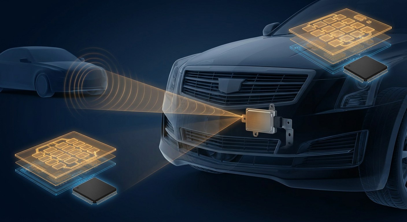
A car with automatic emergency braking does not need to read the number plate of the vehicle in front. It only needs to know that something is 38 metres away, closing at 12 metres per second, and sitting in its own lane. That is the job of the 77 GHz radar fitted to millions of cars over the past decade, and it does it without light, without a camera, and without seeing anything in the usual sense of the word: it transmits a continuous wave whose frequency sweeps up and down, then measures how long it takes to come back as a different frequency.
A frequency ramp instead of a pulse
Early radars worked like sonar: emit a short pulse and time the echo. In a car that is a problem, because measuring 200 metres to centimetre accuracy would need pulses lasting a fraction of a nanosecond and electronics sampling at tens of gigasamples per second. The industry chose another technique, frequency-modulated continuous wave (FMCW) radar, which turns time of flight into a frequency difference that cheap electronics can measure.
The transmitter continuously emits a signal whose frequency rises linearly from 76 to 80 GHz over tens of microseconds. That ramp is called a chirp. The signal travels, bounces off the obstacle and comes back delayed. Meanwhile the local oscillator has kept climbing, so mixing the received signal with the one being transmitted at that instant produces a difference, the beat frequency, which is proportional to the delay and therefore to distance. Nothing has to be timed: a Fourier transform of the mixed signal shows at which frequency the peak appears.
The relationship is simple: range = c · fbeat · T / (2 · B), where c is the speed of light, T the chirp duration and B the swept bandwidth. With a 40-microsecond ramp and 4 GHz of bandwidth, an object at 100 metres returns a beat of about 6.7 MHz, easily digitised by a 20 or 40 megasample-per-second analogue-to-digital converter.
Where resolution comes from
Bandwidth does not only improve accuracy: it sets the ability to separate two objects. Range resolution equals c / (2B). With the 4 GHz allowed in the 77 GHz band that is 3.75 centimetres; with the 200 MHz of the old 24 GHz band, 75 centimetres. That gap is what pushed the whole automotive industry up the spectrum: at 24 GHz two motorbikes half a metre apart merge into a single target, while at 77 GHz they are seen separately.
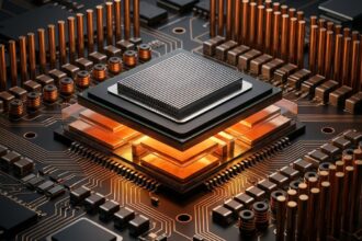
The band is not arbitrary either. The International Telecommunication Union reserved 76 to 81 GHz for automotive radars, on condition that they do not interfere with nearby radio astronomy services. At 79 GHz the wavelength is around 3.8 millimetres, small enough for antennas of that size to be integrated into the chip package itself, with no optics and no glass window.
The second dimension: velocity
A single chirp gives range but does not say whether the car ahead is closing or pulling away. For that the radar transmits a burst of tens or hundreds of consecutive chirps, spaced about 50 microseconds apart. Between one and the next the object has moved and the echo comes back with a Doppler shift. At 77 GHz a relative speed of 1 m/s produces a shift of barely 513 Hz, invisible next to the megahertz of the beat. The fix is to treat each stack of samples as a matrix: a first FFT along the fast dimension (within the chirp) gives range; a second FFT along the slow dimension (across chirps) gives velocity. The result is the range-Doppler map, a two-dimensional image in which every cell says how much reflected energy sits at a given range and speed.
That map is also where ground clutter is separated from vehicles: a static crash barrier appears in the zero-velocity column, while an approaching car falls in another cell, even when both are at the same distance.
Angle, virtual arrays and MIMO
Knowing range and speed is not enough to decide whether to brake: the system has to know which lane the obstacle is in. Angle comes from comparing the phase of the same signal across several receiving antennas spaced half a wavelength apart. The phase difference between two consecutive antennas is proportional to the sine of the arrival angle, and a third FFT dimension yields the range-Doppler-angle map.
Angular resolution depends on the number of antennas and their spacing. That is why modern radars use MIMO (multiple-input multiple-output): with 3 transmitters and 4 receivers, the combinations create a virtual array of 12 elements with a wider aperture than the physical one. Twelve virtual channels give roughly 10 degrees of angular resolution; fourth-generation imaging radars, with cascaded chips and 48 or more channels, get down to 1.5 degrees and produce a near three-dimensional point cloud, close to a lidar’s but with radial velocity included.
What reaches the processor
The radar chip does not deliver objects: it delivers samples. Everything else is digital processing in a DSP or a dedicated microcontroller. The typical chain is: windowing (Hamming or Hann) to reduce spectral leakage, FFT in two or three dimensions, peak detection with a CFAR (constant false alarm rate) detector, which sets its threshold adaptively from the noise in neighbouring cells so it neither fires at a street lamp nor misses a pedestrian, clustering of detections and, finally, a Kalman filter that keeps each object’s identity across cycles and smooths its trajectory.
A current car radar completes that cycle every 30 to 50 milliseconds, with 128 or 256 chirps per burst, which means tens of millions of samples per second on a few watts of power.
Its limits are physics, not software
Radar is robust: it cuts through fog, rain, dust and total darkness, where a camera goes blind. But at 77 GHz almost everything reflects, including wet asphalt and roadside metal signs, and that produces multiple echoes the processor reads as ghost objects. A lorry can produce one target at its height and another below the road surface from a bounce. Telling them apart demands propagation models and a great deal of track validation.
The other problem is mutual interference. With hundreds of millions of radars in circulation, two cars crossing can emit chirps in the same band at the same instant; the foreign signal enters the receiver as correlated noise and lifts the floor of the range-Doppler map. The industry’s answer is randomised chirp sequences, coordinated frequency hopping, and detectors that recognise the interference pattern and mask it before the FFT.
That is why no serious manufacturer relies on radar alone. The trend is sensor fusion: camera to classify, lidar for fine geometry, radar for relative range and speed, with radar as the safety net when the other two degrade. At 120 km/h every extra metre of early detection is 30 more milliseconds of decision time, and that is exactly what separates braking from a crash.