
When an app tells you «products similar to this one», «articles you might like» or «similar images», it is not comparing your selection against every other item row by row. There is a step beforehand that turns each text, image or audio clip into a vector, and a data structure that makes the search almost instantaneous even when the collection holds millions of entries. This article explains how.
From text to numbers: the role of embeddings
A neural network (a model with millions of parameters tuned on example data) can turn any item into an embedding: a list of hundreds of real numbers that summarises its meaning. Two texts with a similar sense end up producing embeddings whose numbers land close together in that high-dimensional space.
The closeness between two vectors is measured with cosine similarity, the cosine of the angle between them: it is 1 when they point in the same direction and 0 when they are perpendicular. It is cheap to compute, but there is a catch: searching it literally over N vectors costs N comparisons, and with millions of documents that becomes slow.
The naive search and its real cost
Comparing a query vector against each of the N stored ones is a linear scan: walking the whole table. If each comparison costs D operations (the embedding dimension), the total cost is O(N·D). With ten million documents and 384-dimensional vectors we are talking about billions of operations per query; far too many to answer in milliseconds.
To speed it up, a little accuracy is traded away: the idea is to return the nearest neighbours approximately, without a strict mathematical guarantee. That is why this family of techniques is called ANN (approximate nearest neighbour).
HNSW: the graph that jumps between layers
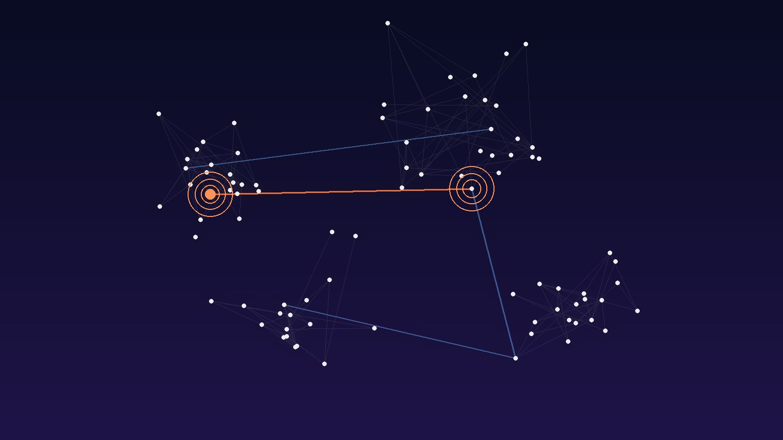
The most popular index today, HNSW (Hierarchical Navigable Small World), turns the vectors into nodes of a graph — a set of points joined by edges — arranged in several layers. The upper layers hold few nodes with long edges; the lower layers hold every node with short connections.
The search starts at the top and works its way down: on each layer it hops from node to node towards the ones closest to the query and, when it hits a local minimum, descends to the next layer. Because the upper layers act as long-range shortcuts, the route stays short however huge the graph. The result is that queries over millions of vectors drop to a few milliseconds.
A 90-degree entry: quantisation
To use less memory and compare even faster, quantisation is applied: representing each vector with less precision, for example turning every 32-bit number into an 8-bit code. Accuracy is lost, but more vectors fit in RAM and the CPU handles each comparison more quickly.
Why the architecture matters
A vector database (such as Qdrant, Milvus or Weaviate) combines this index with the classic machinery of a store: persistence, metadata filters, replicas and versioning. The index lives in memory to stay fast and is updated incrementally as new data arrives.
Understanding this layer explains two things. First: performance depends on the embedding dimensionality and the graph’s branching factor, not just on the hardware. Second: similarity search is approximate, and in applications where a mistake is expensive — such as confirming an identity — it pays to add an exact re-ranking pass after the index.